Detecting Traffic Flow

In this paper by Bing Yu, Haoteng Yin, and Zhanxin Zhu, researchers from the Beijin Institute of Big Data Research and Center for Data Science from Peking University try to use a spatial-temporal graph convolutional network to tackle time series prediction.

The authors claim that impractical assumptions and simplifications degrade prediction accuracy of medium and long term (30 minutes into the future) traffic prediction. The problem is formally described as

Traffic forecast is a typical time-series prediction problem, i.e. predicting the most likely traffic measurements (e.g. speed or traffic flow) in the next H time steps given the previous M traffic observations as:

\(\hat{v_{t+1}}, ...., \hat{v_{t+H}} = \text{argmax}_{v_{t+1},...,v_{t+H}} \text{log} P(v_{t+1},...,v_{t+H}|v_{t-M+1},...,v_{t})\)

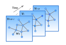
where \(v_{t} \in \mathbb{R}^{n}\) is an observation vector of n road segments at time step t, each element of which records historical observation for a single road segment.

Interestingly, due to the way they chose to structure the data, their weighted adjacency matrix \(W \in \mathbb{R}^{n x n}\), which could require a large amount of memory.

Defining a convolution on a graph:

This paper re-introduced the idea of convolutions on graph. They use the standard definition of the convolution:

where L is the normalized graph Laplacian is defined as \(L = I_{n} - D^{-\frac{1}{2}} W D^{-\frac{1}{2}} = U\Lambda U_{T} \in \mathbb{R}^{n x n}\). The Laplacian is a symmetric matrix, so it is guaranted to be diagonalizable and \(\Lambda \in \mathbb{R}^{n x n}\) is the diagonal matrix of eigenvalues of L. The paper by Kipf and Welling introduces this operation in 2016. ¹

Architecture:

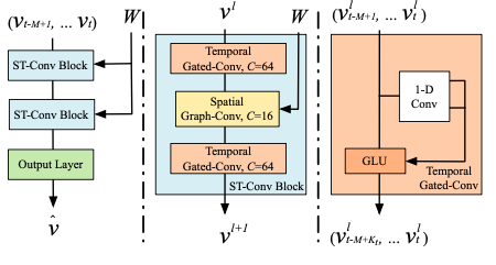
The proposed architecture of the STGCN is comprised of two gated convolutional layer with one spatial graph convolutional layer nested between them as can be seen in the second block of the figure below.

In Tensorflow, the implementation of the convolutional layers is pretty easy to use ² i.e.

def _build(self):

        self.layers.append(GraphConvolution(input_dim=self.input_dim,
                                            output_dim=FLAGS.hidden1,
                                            placeholders=self.placeholders,
                                            act=tf.nn.relu,
                                            dropout=True,
                                            sparse_inputs=True,
                                            logging=self.logging))

        self.layers.append(GraphConvolution(input_dim=FLAGS.hidden1,
                                            output_dim=self.output_dim,
                                            placeholders=self.placeholders,
                                            act=lambda x: x,
                                            dropout=True,
                                            logging=self.logging))

The authors claim that due to the graph Fourier basis, convolutions through matrix multiplications can be expensive since they’re \(O(n^{2})\), so they use two approximations to speed up calculations.

1. Chebyshev Polynomial Approximations:

The Chebyshev Polynomial Approximations are not only a way to estimate a function’s values over a specific range, but the calculated coefficients give you a great way to get a sense of the maximum range of the error. I found an awesome article by Jason Sachs² who works in embedded systems and the improvement that Chebyshev approximations have over Taylor polynomial approximations, look-up tables, and look-up tables with linear approximation for use cases in approximating values within a specific range.

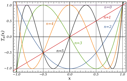
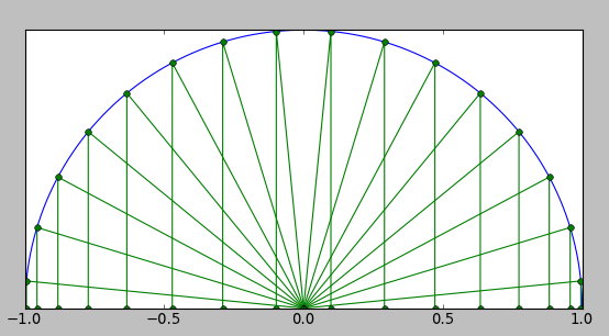
Instead of thinking polynomials as linear combinations of \(1, x, x^{2}, x^{3}\), we can think of them as linear combinations of Chebyshev polynomials \(T_{n}(x) = cos(n cos^{-1}(x))\). Using this mapping, we can generally take a function over a range and map it to the interval \(u \in [-1, 1]\). There is a cool graphical picture of what this looks like that has a Fourier-esque taste to it.

The authors claim that a paper by Defferrard et al. 2016³ can be used to filter equation \((1)\) above to \(O(K\lvert E \rvert)\) where \(K\) is the support size and \(E\) are the edges in the filter. The authors argue that the decomposition from equation \((1)\) can be by rescaling the matrix of eigenvalues \(\hat{\Lambda} = \frac{2\Lambda}{\lambda_{max}} - I_{n}\). Using this re-scaling, we can re-write equation \((1)\) as:

where \(T_{k}(\widetilde{L}) \in \mathbb{R}^{n \times n}\) is the Chebyshev polynomial of order k that has been scaled/approximated.

2. 1st order Approximations:

The authors further claim that

Due to the scaling and normalization in neural networks, we can further assume that \(\lambda_{max} \approx 2\). Thus, equation \((2)\) can further be simplified to:

where \(\theta_{0}\) and \(\theta_{1}\) are two shared kernel parameters, which they then say you can replace with a single parameter \(\theta\) by letting \(\theta = \theta_{0} = -\theta_{1}\) and by renormalizing \(W\) and \(D\) such that \(\widetilde{W} = W + I_{n}\) and \(\widetilde{D_{ii}} = \sum_{j}\widetilde{W}_{ij}\). Then the graph convolution can be further simplified to:

Generalizing Graph Convolutions:

One of the highlights of the paper is that the authors generalize the GCN by bringing up a general case, whereby they add another channel \(C_{i}\) such that instead of being applied only to vectors \(x \in \mathbb{R}^{n}\), they can use multi-dimensional tensors \(X \in \mathbb{R}^{n \times C_{i}}\) where \(C_i\) is the number of channels in a signal. They generalize equation \((1)\) to the following:

where \(C_i \times C_0\) are the standard vectors of Chebyshev coefficients and \(C_i\), \(C_0\) are the size of the input and output feature maps. With regards to the traffic problem, each frame \(v_t\) is a matrix whose columns are considered to be \(C_i\), making their multi-dimensional vector \(X \in \mathbb{R}^{n \times C_i}\).

Gated CNNs for Extracting Temporal Features:

The authors argue that although RNNs are good for modeling time-series, they are difficult to train. Their architecture is described below with

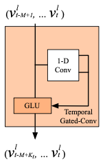
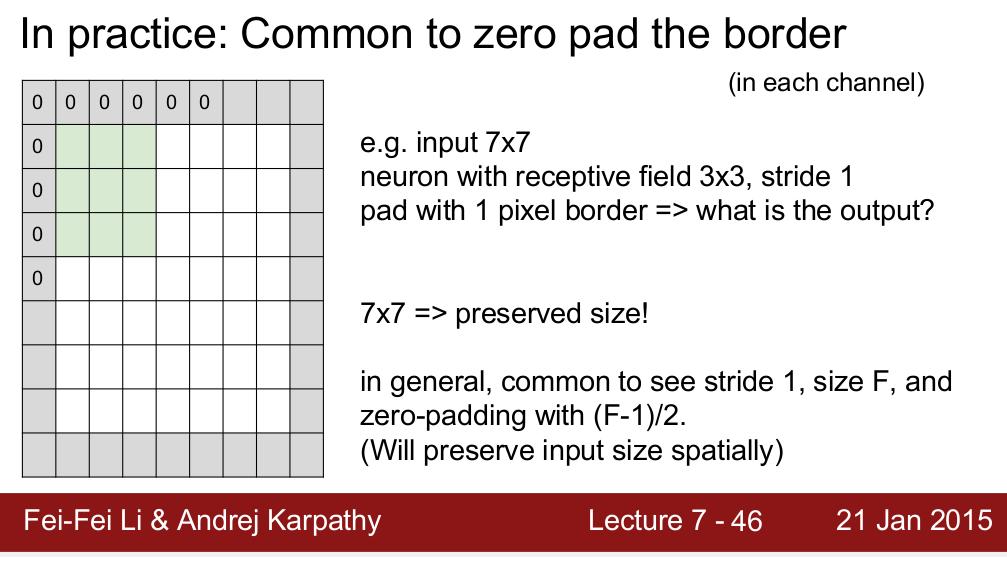
After reading about the architecture not using padding after application of the 1-d convolution with width - \(K_t\) kernel, I looked up some opinions on padding in general⁴ and the general consensus seems to be in order to preserve the spatial size.

The dimensions of the temporal convolution for each node represented by the arrow with two outputs from the 1-D conv in the figure below taking in inputs of length - \(M\) with \(C_i\) channels as described before (\(Y \in \mathbb{R}^{M \times C_i}\)) and multiplies it by a convolution kernel \(\Gamma \in \mathbb{R}^{K_t \times C_i \times 2C_0}\) and maps the input:

The authors also mention that they choose to use residual connections between the stacked convolutional layers which strangely is not drawn on their architecture page.

where \(P, Q\) are input to the GLU gates and \(\odot\) is the element-wise Hadamard product.

The answer for the bountied question had an interesting explanation besides the intuitive reasons (easier to design the network/ allows deeper network architectures), that padding improved performance by keeping information at the borders. Although most of the comments were in reference to CNNs for image object detection and identification, it seemed relevant given that the architecture for this STGCN chose not to use padding.

Interestingly, from the source code, it looks like the dimension reductionality is a feature of their architecture where they tried to reduce the output layer size.

Spatio-temporal Convolutional Block:

I found this section to be the most challenging to understand since some of the terms were unfamiliar to me. Also, I was a little bit confused by the dimensions of the inputs and outputs. For example, in the section previously, I thought the output of the temporal convolutional blocks were two dimensional given equation \((6)\), but the paper said that:

The input and output of ST-Conv blocks are all 3-D tensors.

which leads me to believe that the original input to the temporal convolutional layers were 3D and not 2D. This appears to follow from their source code docstring for the spatial convolution layer:

def spatio_conv_layer(x, Ks, c_in, c_out):
    '''
    Spatial graph convolution layer.
    :param x: tensor, [batch_size, time_step, n_route, c_in].
    :param Ks: int, kernel size of spatial convolution.
    :param c_in: int, size of input channel.
    :param c_out: int, size of output channel.
    :return: tensor, [batch_size, time_step, n_route, c_out].
    '''

For an input velocity vector \(v^l \in \mathbb{R}^{M \times n \times C^l}\), we can see the input and output should be the same size. The equation they have for the spatio-temporal convolutional blocks computes:

where \(\Gamma_0^l, \Gamma_1^l\) are the upper and lower temporal kernel. It is interesting to me that they chose to apply the ReLU only to the first temporal kernel. The final output layer (left bottom of figure 1) \(Z \in \mathbb{R}^{n \times c}\) yields the speed predictions for \(n\) nodes. Interestingly, they choose to apply a linear transformation across the \(c\)-channels where \(\hat{v} = Zw + b\). They use the L2 loss to measure the performance of the model where:

Conclusions:

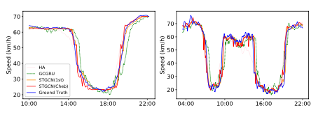
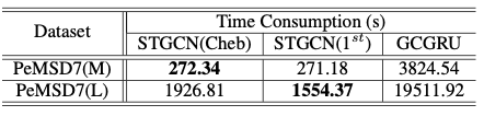
The authors claim that the model architecture allows universal processing of structured time series and is fast because of its use of convolutions instead of recurrent blocks. They choose to use mean absolute errors (MAE) and Mean absolute percentage errors (MAPE) amd show an improvement with both the unmodified and approximated Chebyshev model on the task

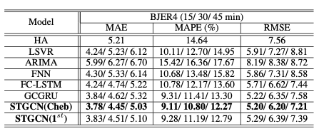
The most impressive improvement that the authors present over the next best model is the amount of time training on the dataset required with comparable errors:

I am looking forward to reading the Kipf and Welling 2016 paper as the architecture for any graph convolutional neural network will probably use the formulation that they proposed or a closely related variant. There’s also an interesting book called Numerical Recipes ⁵ that I would be interested in checking out when I have some more free time to look at some more ways to apply number theory to speeding up calculations. The book is also available for free online as a PDF, so even more reason to check it out and support the author. The first chapter hit a ton of topics that I was introduced to in linear algebra including Gauss-Jordan Elimination, LU Decomposition, SVD, QR Decomposition, and some topics that I have personally never heard about it which is kind of exciting. (There is a section called “Is Matrix Inversion an \(N^{3}\) Process” which I find pretty cool.)

• 2023 1
• 2022 2